Introduction
Random forests are known as ensemble learning methods used for classification and regression, but in this particular case I'll be focusing on classification. Random forests are essentially a collection of decision trees that are each fit on a subsample of the data. While an individual tree is typically noisey and subject to high variance, random forests average many different trees, which in turn reduces the variability and leave us with a powerful classifier.
Random forests are also non-parametric and require little to no parameter tuning. They differ from many common machine learning models used today that are typically optimized using gradient descent. Models like linear regression, support vector machines, neural networks, etc. require a lot of matrix based operations, while tree based models like random forest are constructed with basic arithmetic. In other words, to build a tree all we're really doing is selecting a hand full of observations from out dataset, picking a few features to look through, and finding the value that makes the best split in our data. We'll define what what it means to be the "best split" in a bit..
Decision Trees
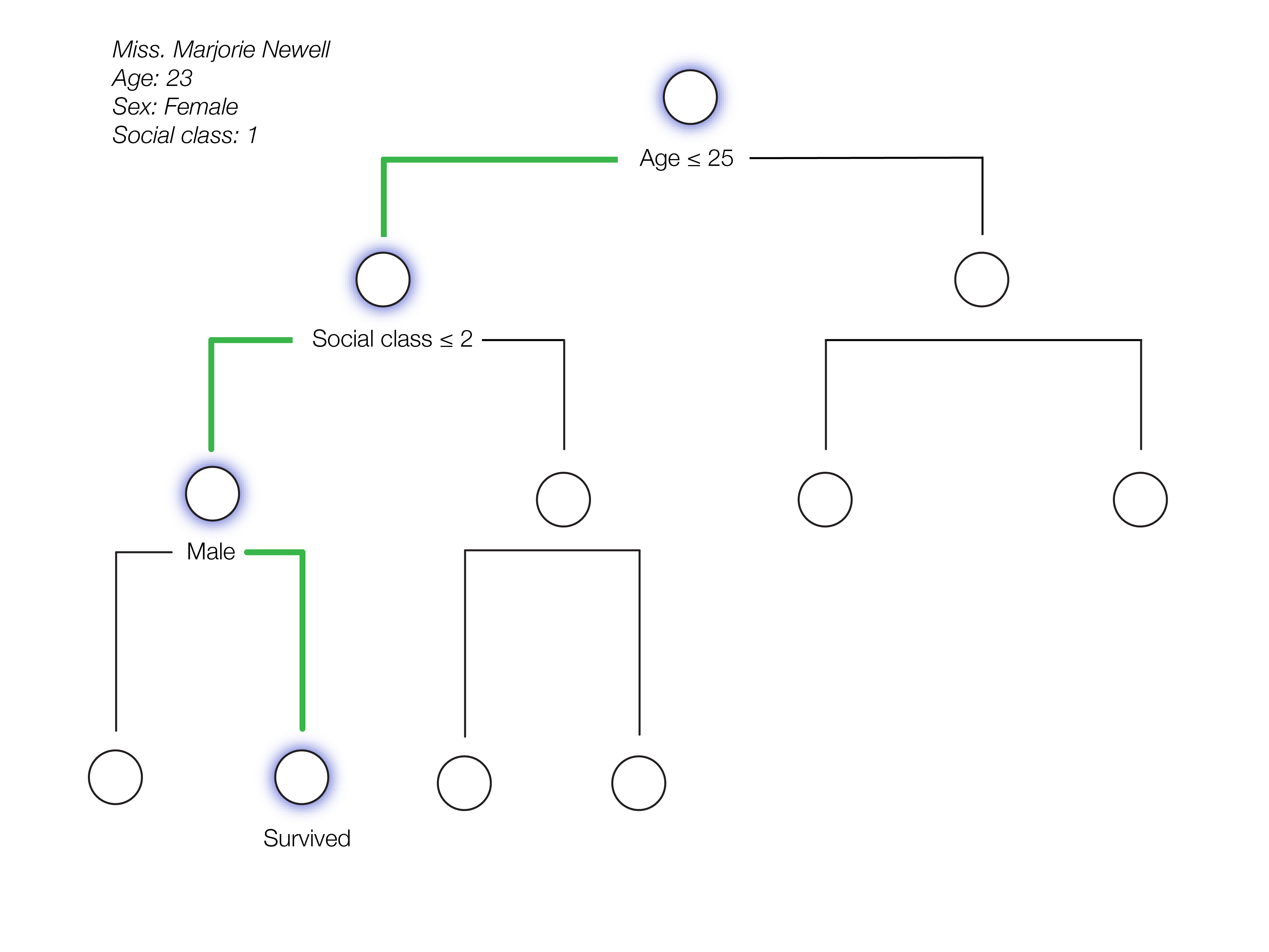
A quick overview if you're not familiar with binary decision trees. We start from very top, which we'll call the root node, and ask a simple question. If the answer to the question is correct we'll move to the left node directly connected below, which we'll call the left child, otherwise, if the answer is wrong we'll move down to the right node, which we'll call the right child. We'll repeat this process until we reach one of the bottom nodes, also known as the terminal nodes. For classification the terminal nodes output the class that is the mode while in the context of regression they'll output the mean prediction.
The problem with relying on a single tree is that it needs a lot of depth to gain strong predictive power. Binary decision trees can have up to size $2^{d+1}-1$, where $d$ is the depth of the tree, so for example, a tree with a depth of 10 can ask up to 2047 different questions. This ultimately leads to a lot of complexity within our tree and in the world of machine learning high complexity leads to high variance. The image below illustrates the problem with an individual decision tree having high variance.
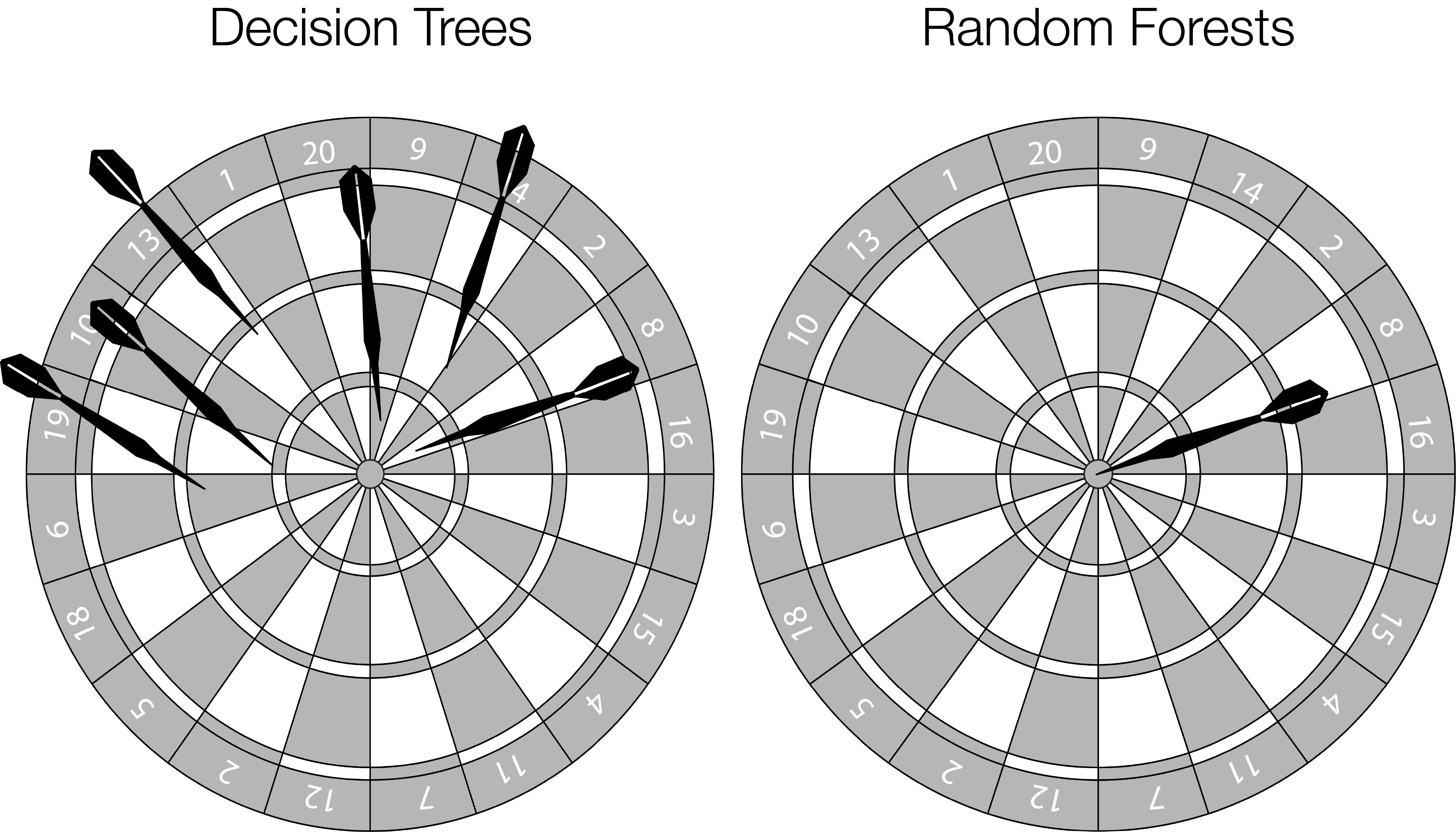
Decision trees have whats called low bias and high variance. This just means that our model is inconsistent, but accurate on average. Imagine a dart board filled with darts all over the place missing left and right, however, if we were to average them into just 1 dart we could have a bullseye. Each individual tree can be thought of as the innacurate darts and a random forest would give us that bullseye.
The Data
In this particular example I'll be using Kaggles Titanic dataset. This dataset is incredibly simple and will be useful for demonstrating how the model works in its entirety.
import random
import pandas as pd
import numpy as np

df = pd.read_csv('../data/train.csv')
df.head()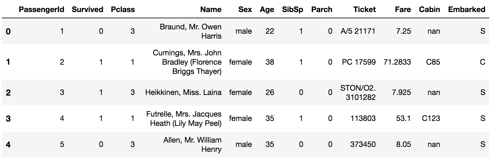
The datast consists of simple attributes for each passenger like their age, sex, social class, # of family members, and where they embarked. The objective is to predict whether a passenger survived the titanic crash or not, where 1 denotes that the passenger survived and 0 denotes that they perished.
Something important to note is that random forests don't handle missing values. This will require some preprocessing steps before training a model if there's any missing data. For simplicity I will just be replacing any missing values with the features avarage or mode. I'm not going to dwell on the details of this dataset, so if you're interested in learning more about it I would highly recommend looking over kernels within the competition.
df.loc[df['Age'].isnull(),'Age'] = np.round(df['Age'].mean())
df.loc[df['Embarked'].isnull(),'Embarked'] = df['Embarked'].value_counts().index[0]
In this example I'm going to be using the 7 features: Pclass, Sex, Age, SibSp, Parch, Fare, Embarked
Lets split the data into a training and testing set so we'll be able to validate our models performance
features = ['Pclass','Sex','Age','SibSp','Parch', 'Fare', 'Embarked']
nb_train = int(np.floor(0.9 * len(df)))
df = df.sample(frac=1, random_state=217)
X_train = df[features][:nb_train]
y_train = df['Survived'][:nb_train].values
X_test = df[features][nb_train:]
y_test = df['Survived'][nb_train:].values
Entropy
The most commonly used measurements for constructing binary decision trees are: Entropy, Classification Error, and Gini index. In this thread we'll be focusing on entropy, which a measurement of uncertainty (sometimes called impurity) that uses the following formula
$$H(X) = -\sum_{j}p_j\log p_j$$
such that $p_j$ is the probability of class $j$.
At first glance this formula might not make any sense, but once we see some examples it actually has some great properties. In the case of binary classification entropy takes on the form
$$H(X) = -p\log_2p-(1-p)\log_2(1-p)$$
where $p$ denotes $P(X=1)$ (the probablity that a passenger survived). Also note that in the case of binary classification we use $\log_2$, agian we'll see more about this in a bit
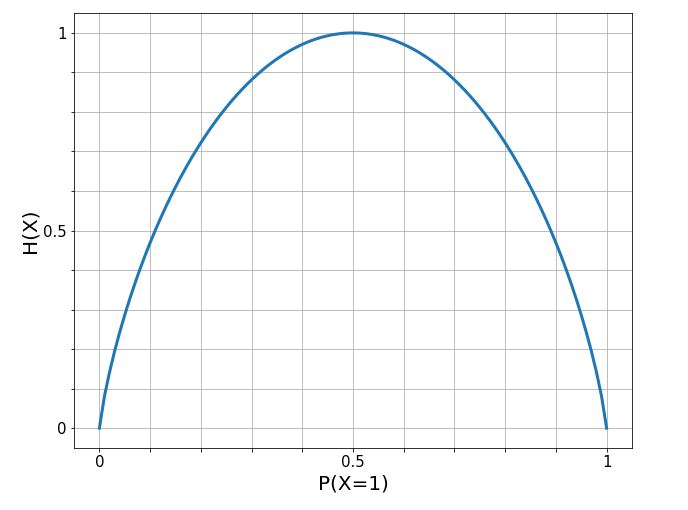
Entropy follows a very intuitive interpretation with the following properties:
- Certainty: Entropy is minimized when all samples in a node belong to the same class such that $P(X=1) = 1$ (in our case every passenger survives)
- $-1\log_2(1) - 0\log_2(0) = 0$
- Uncertainty: Entropy is maximized when we a uniform class ditrubution such that $P(X=1)$ = 0.5 (in our case each passenger has a 50% chance of surviving)
- $-0.5\log_2(0.5) - 0.5\log_2(0.5) = 0.5 + 0.5 = 1$
Information Gain
When we compare the entropy from before and after a split we get whats called information gain. Information gain measures how much information we gained when splitting a node at a particular value. Information gain $IG$ is computed with the following formula, $$IG(D)=I(D_p)-\frac{N_{left}}{N_p}I(D_{left})-\frac{N_{right}}{N_p}I(D_{right})$$ where $D_p, D_{left}, D_{right}$ represent the datasets from the parent, left, and right children nodes, $N_p$, $N_{left}$, $N_{right}$ represent the number of observations in the parent, left and right children nodes and $I(D)$ denotes the entropy for that particular node. This formula can be intrepreted as $$\text{information gain} = \text{entropy}_{\text{before}} - \text{entropy}_{\text{after}}$$ where $\text{entropy}_{\text{before}}$ is a measure of how uncertain we were with our data before we made the split and $\text{entropy}_{\text{after}}$ is a measure for how uncertain we are after we split the data. We'll always want to split a node with the value that maximizes information gain. Let's look at an example to make this concept of entropy and information gain more concrete.
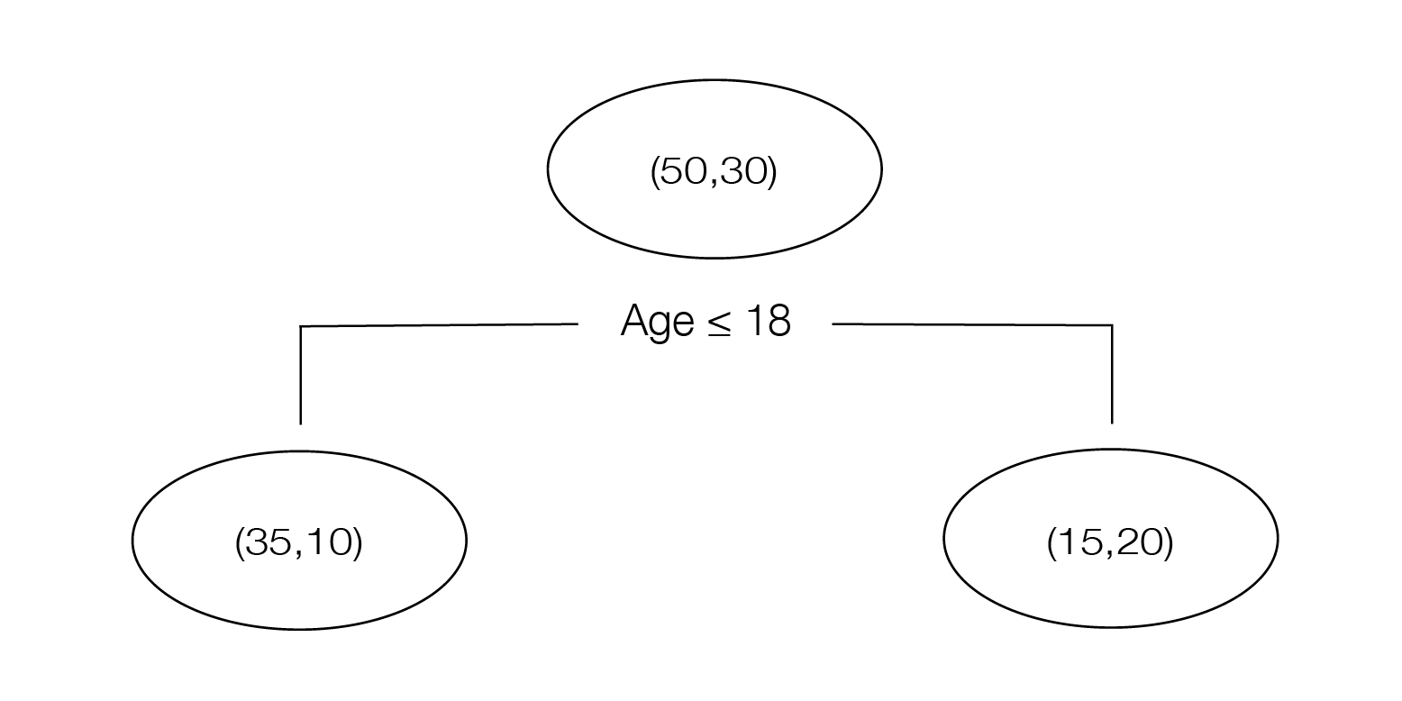
In this example the parent node has 80 total passengers, 50 survived, and 30 perished. All passengers 18 years old or younger drop into the left child (35 survived, 10 perished) and all passengers older than 18 drop into the right child (15 survived, 20 perished). If we compute the entropy for the parent and both children nodes we'll have the following: $$I(D_p) = -\frac{30}{80}\log_2(\frac{30}{80})-\frac{50}{80}\log_2(\frac{50}{80}) = 0.95$$ $$I(D_{left}) = -\frac{25}{35}\log_2(\frac{25}{35})-\frac{10}{35}\log_2(\frac{10}{35}) = 0.86$$ $$I(D_{right}) = -\frac{5}{45}\log_2(\frac{5}{45})-\frac{40}{45}\log_2(\frac{40}{45}) = 0.50$$ which will give us the following information gain, $$I(D) = 0.95 - \frac{35}{80}(0.86)-\frac{45}{80}(0.50) = 0.292$$ If this is the largest information gain among all the possible splits we would use this value as the chosen split point on this particular node. We'll repeat this process for each node until we've reached a terminal node that only consists of one class only or when we reach the maximum depth specified beforehand. The class with the highest counts in a terminal node (sometimes referred to as a leaf) will be assigned to any test value that lands on that terminal. Now that we know how to construct a single tree lets go over the method for building a random forest..
Bootstrapping
One of the main reasons random forests are so powerul is due to the randomness injected into each tree. What do I mean by this?
Each individual decision tree will be constructed on a bootstrapped subset of our data. If our dataset has $n$ observations bootstrapping is the process of sampling $n$ points with replacement. This means that some obsverations in our data set will be selected more than once and some won't be selected at all. We can actually calculate that the probability an observation is omitted from our bootstrapped dataset is $(1 - \frac{1}{n})^{n}$. By definition $e^{-1} = \displaystyle \lim_{n\to\infty}(1-\frac{1}{n})^n$ and since $e^{-1}$ = 0.36787.. $\approx \frac{1}{3}$ $\Rightarrow$ bootstrapping $n$ samples with replacement will leave out approximately $\frac{1}{3}$ of the observations in each distinct tree. Since each individual tree is built using only $\frac{2}{3}$ of the data we'll find that most trees will differ significantly from one another. If interested, a full proof of this can be found on my blog here.
The other great thing that comes with bootstrapping is that we get whats called an out-of-bag error estimate for free. The OOB (out-of-bag) samples are the $\approx \frac{1}{3}$ observations that were not selected to build a parcticular tree. Once we've built our tree with the n bootstrapped observations we can test each $\vec{x}_i$ that was left out and compute the mean prediction error from those samples. We can compute an OOB score for each tree and take the average of all those scores to get an estimate for how accurate our random forests performs, this is essentially leave-one-out cross validation. This will give us an estimate for how accurate our model is without having to formally test it on new data and we'll soon find that it is approximately the same error rate we'll get at test time.
Bagging
The other great idea that random forests introduce is the concept of bagging. Bagging is the process of growing a tree where each node in the tree looks at every value in our bootstrapped sample in every feature to find the best split in the data at that particular node. This is repeated for all trees.
Random forests follow the same procedure as bagging, however, the key difference is that on a dataset with $p$ features each tree will only look at a subset of $m$ features where $m=\sqrt(p)$. This is injecting even more randomness into the model due to the fact that if we sampled all $p$ features in each tree we would likely be making splits at the same values from the same features in most trees. Given that we are only looking at $\sqrt(p)$ features at one time many of the trees will look at a different groups of feature from one another. With this we'll be able to produce many *uncorrelated* trees which will help us capture a lot of the variability as well as interactions between multiple variables.
Random Forest Algorithm
Suppose we have the following data data {$(\vec{x}_1,y_1),(\vec{x}_2,y_2),..,(\vec{x}_n,y_n)$} where each $\vec{x}_i$ represents a feature vector $[x_{i1},x_{i2},...,x_{im}]$ and let $B$ be the number of trees we want to construct in our forest. We will do the following,
- for $b=1$ to $B$:
- Draw a bootstrap sample of size n from the data
- Grow a decision tree $T_b$ from our bootstrapped sample, by repeating the following steps until the each node consists of 1 class only or until we've reached the minimum node size $\min_{size}$ specified beforehand
- sample $m=\sqrt{p}$ features (where $p$ is the number of features in our dataset)
- compute the information gain for each possible value among the bootstrapped data and $m$ features
- split the node into 2 children nodes
- Output the ensemble of trees $\{T\}^B_1$
Show Me The Code
Now that we understand how to construct an individual decision tree and all the necessary steps to build our random forest lets write it all from scratch in python.
Lets first define entropy and information_gain which we will help us in finding the best split point
def entropy(p):
    if p == 0:
        return 0
    elif p == 1:
        return 0
    else:
        return - (p * np.log2(p) + (1 - p) * np.log2(1-p))

def information_gain(left_child, right_child):
    parent = left_child + right_child
    p_parent = parent.count(1) / len(parent) if len(parent) > 0 else 0
    p_left = left_child.count(1) / len(left_child) if len(left_child) > 0 else 0
    p_right = right_child.count(1) / len(right_child) if len(right_child) > 0 else 0
    IG_p = entropy(p_parent)
    IG_l = entropy(p_left)
    IG_r = entropy(p_right)
    return IG_p - len(left_child) / len(parent) * IG_l - len(right_child) / len(parent) * IG_r
where entropy takes in a probability of a class within a node and information_gain takes in a list of the classes from the left and right child and returns the information gain of that particular split.
Lets also define a draw_bootstrap function that can take in the training input $X$ in the form of a dataframe and also the output $y$ in the form of an array. We'll have it return the bootstrap sampled $X_{boot}$ and $y_{boot}$ that we'll use to construct a tree. We'll also return the out-of-bag observations that were left out for training which we'll call X_oob andy_oob. At each new iteration we'll use the OOB samples to evaluate the performance of the tree built with the bootstrapped data. So in other words, if we have 100 trees we'll have 100 OOB scores
def draw_bootstrap(X_train, y_train):
    bootstrap_indices = list(np.random.choice(range(len(X_train)), len(X_train), replace = True))
    oob_indices = [i for i in range(len(X_train)) if i not in bootstrap_indices]
    X_bootstrap = X_train.iloc[bootstrap_indices].values
    y_bootstrap = y_train[bootstrap_indices]
    X_oob = X_train.iloc[oob_indices].values
    y_oob = y_train[oob_indices]
    return X_bootstrap, y_bootstrap, X_oob, y_oob

def oob_score(tree, X_test, y_test):
    mis_label = 0
    for i in range(len(X_test)):
        pred = predict_tree(tree, X_test[i])
        if pred != y_test[i]:
            mis_label += 1
    return mis_label / len(X_test)
Next we'll define find_split_point which does the following:
- select $m$ features at random
- for each feature selected, iterate through each value in the bootstrapped dataset and compute the information gain
- Return a dictionary from the value that gives the highest information gain, which will represent a node in our tree consisting of:
- (int) the feature index
- (int) the value to split at
- (dictionary) left child node
- (dictionary) right child node
X_bootstrap and outputs $y_{boot}$ as y_bootstrap
def find_split_point(X_bootstrap, y_bootstrap, max_features):
    feature_ls = list()
    num_features = len(X_bootstrap[0])

    while len(feature_ls) <= max_features:
    feature_idx = random.sample(range(num_features), 1)
    if feature_idx not in feature_ls:
        feature_ls.extend(feature_idx)

    best_info_gain = -999
    node = None
    for feature_idx in feature_ls:
    for split_point in X_bootstrap[:,feature_idx]:
        left_child = {'X_bootstrap': [], 'y_bootstrap': []}
        right_child = {'X_bootstrap': [], 'y_bootstrap': []}

        # split children for continuous variables
        if type(split_point) in [int, float]:
            for i, value in enumerate(X_bootstrap[:,feature_idx]):
                if value <= split_point:
                    left_child['X_bootstrap'].append(X_bootstrap[i])
                    left_child['y_bootstrap'].append(y_bootstrap[i])
                else:
                    right_child['X_bootstrap'].append(X_bootstrap[i])
                    right_child['y_bootstrap'].append(y_bootstrap[i])
        # split children for categoric variables
        else:
            for i, value in enumerate(X_bootstrap[:,feature_idx]):
                if value == split_point:
                    left_child['X_bootstrap'].append(X_bootstrap[i])
                    left_child['y_bootstrap'].append(y_bootstrap[i])
                else:
                    right_child['X_bootstrap'].append(X_bootstrap[i])
                    right_child['y_bootstrap'].append(y_bootstrap[i])

        split_info_gain = information_gain(left_child['y_bootstrap'], right_child['y_bootstrap'])
        if split_info_gain > best_info_gain:
            best_info_gain = split_info_gain
            left_child['X_bootstrap'] = np.array(left_child['X_bootstrap'])
            right_child['X_bootstrap'] = np.array(right_child['X_bootstrap'])
            node = {'information_gain': split_info_gain,
                    'left_child': left_child,
                    'right_child': right_child,
                    'split_point': split_point,
                    'feature_idx': feature_idx}


    return node
We'll next need a function that decides when to stop splitting nodes in a tree and finally output a terminal node (classifies whether the passenger survives or perishes). On a single tree split_node works as follows:
-
Given a node, store the left and right children as
left_child&right_childand remove them from the original dictionary -
Check if either children has 0 observations in them. If one of the children is entirely empty this ultimately means that the best split in the data for that node was unable to differentiate the 2 classes and its best to call
terminal_nodeand return the tree.terminal_nodereturns the class with the highest counts at the current node. - Check if the current depth of the tree has reached the maximum depth. If so, create a terminal node and return the tree
-
Check if number of observations in the left child at the current node is less than the minimum samples needed to make a split, which will be stored as
min_samples_split. If so create a terminal node and return the tree -
If the left child has more observations than
min_samples_splitwe'll feed that left node intofind_split_pointagain to find the best split point and repeat steps 1 - 6. This is ultimately going to be nesting dictionaries, which we are using to represent each node in our tree. - Repeat steps 4 and 5 for the right child node
- Repeat steps 1 - 6 until each branch has a terminal node
def terminal_node(node):
    y_bootstrap = node['y_bootstrap']
    pred = max(y_bootstrap, key = y_bootstrap.count)
    return pred


def split_node(node, max_features, min_samples_split, max_depth, depth):
    left_child = node['left_child']
    right_child = node['right_child']

    del(node['left_child'])
    del(node['right_child'])

    if len(left_child['y_bootstrap']) == 0 or len(right_child['y_bootstrap']) == 0:
        empty_child = {'y_bootstrap': left_child['y_bootstrap'] + right_child['y_bootstrap']}
        node['left_split'] = terminal_node(empty_child)
        node['right_split'] = terminal_node(empty_child)
        return

    if depth >= max_depth:
        node['left_split'] = terminal_node(left_child)
        node['right_split'] = terminal_node(right_child)
        return node

    if len(left_child['X_bootstrap']) <= min_samples_split:
        node['left_split'] = node['right_split'] = terminal_node(left_child)
    else:
        node['left_split'] = find_split_point(left_child['X_bootstrap'], left_child['y_bootstrap'], max_features)
        split_node(node['left_split'], max_depth, min_samples_split, max_depth, depth + 1)
    if len(right_child['X_bootstrap']) <= min_samples_split:
        node['right_split'] = node['left_split'] = terminal_node(right_child)
    else:
        node['right_split'] = find_split_point(right_child['X_bootstrap'], right_child['y_bootstrap'], max_features)
        split_node(node['right_split'], max_features, min_samples_split, max_depth, depth + 1)
Parameters
- n_estimators: (int) The number of trees in the forest.
- max_features: (int) The number of features to consider when looking for the best split (typically $\sqrt(p)$
- max_depth: (int) The maximum depth of the tree
- min_samples_split: (int) The minimum number of samples required to split an internal node
To build a single tree we'll need the $X_{boot}$ and $y_{boot}$ values from our bootstrapped data along with the max_depth, min_samples_split, and max_features parameters. We first call find_split_point to create the very first split in our tree which we'll call *root_node*. Once we have a root node we can feed it into split_node which will recusively split each internal node until each branch has a terminal node.
Now that we can build a single tree we can finally build our random forest which will just be a collection of these trees. When we call random_forest we'll need to specify n_estimators, max_features, max_depth, min_samples_split. Then for each tree we've built we'll use all the observations left out of our bootstrapped data to get our OOB score and append it on to a list (I'll talk about how to compute the OOB score and predict on a single tree below). Once we've built n_estimators trees we can print the mean OOB score and return the full list of trees which will represent our ensemble.
def build_tree(X_bootstrap, y_bootstrap, max_depth, min_samples_split, max_features):
    root_node = find_split_point(X_bootstrap, y_bootstrap, max_features)
    split_node(root_node, max_features, min_samples_split, max_depth, 1)
    return root_node

def random_forest(X_train, y_train, n_estimators, max_features, max_depth, min_samples_split):
    tree_ls = list()
    oob_ls = list()
    for i in range(n_estimators):
        X_bootstrap, y_bootstrap, X_oob, y_oob = draw_bootstrap(X_train, y_train)
        tree = build_tree(X_bootstrap, y_bootstrap, max_features, max_depth, min_samples_split)
        tree_ls.append(tree)
        oob_error = oob_score(tree, X_oob, y_oob)
        oob_ls.append(oob_error)
    print("OOB estimate: {:.2f}".format(np.mean(oob_ls)))
    return tree_ls
Given a input vector $\vec{x}_i$ we can predict its class given a single tree with predict_tree. As a single tree consists of nested dictionaries which each represent a node we can let our $\vec{x}_i$ flow through a tree by constantly checking if the split we're at contains another dictionary (node). Once we reach a left_split or right_split that does not contain any dictionary we've reached the terminal node and we can return the class.
def predict_tree(tree, X_test):
    feature_idx = tree['feature_idx']

    if X_test[feature_idx] <= tree['split_point']:
        if type(tree['left_split']) == dict:
            return predict_tree(tree['left_split'], X_test)
        else:
            value = tree['left_split']
            return value
    else:
        if type(tree['right_split']) == dict:
            return predict_tree(tree['right_split'], X_test)
        else:
            return tree['right_split']
We'll repeat the above process for an input $\vec{x}_i$ for all the trees in our ensemble and whichever class was returned more frequently will be the class predicted from our model.
def predict_rf(tree_ls, X_test):
    pred_ls = list()
    for i in range(len(X_test)):
        ensemble_preds = [predict_tree(tree, X_test.values[i]) for tree in tree_ls]
        final_pred = max(ensemble_preds, key = ensemble_preds.count)
        pred_ls.append(final_pred)
    return np.array(pred_ls)
Now that we have our model built we can fit it to our training data with random_forest and predict on our training data
n_estimators = 100
max_features = 3
max_depth = 10
min_samples_split = 2

model = random_forest(X_train, y_train, n_estimators=100, max_features=3, max_depth=10, min_samples_split=2)
OOB estimate: 0.22
preds = predict_rf(model, X_test)
acc = sum(preds == y_test) / len(y_test)
print("Testing accuracy: {}".format(np.round(acc,3)))
Testing accuracy: 0.768
Conclusion
I hope this was of use for anyone curious to learn about random forests. Random forests are great for an array reasons that include an easy implementation and require little to no parameter tuning. RF's may not be power houses like neural networks or gradient boosting models, but they should certainly be in everyones machine learning repertoire. There are methods that can allow you to see which variables are more important than others that I didn't cover in this thread, but are worth looking into. Hopefully this can also help you get in the right direction if you are also interested in understanding how gradient boosting models like Xgboost work.